Optimal Path Planning for Wheeled Robots

1 Introduction

This article first rigorously formulates the optimal control problem (OCP) of finding the shortest path connecting two points through an obstacle field for a non-holonomic car. It then focuses on solving the problem numerically. This is a bit tricky due to the non-differentiability of the cost functional and the presence of so-called “active arcs” in the optimal solution, which results in control chattering. We will see how these numerical difficulties can be dealt with through some easy tricks.

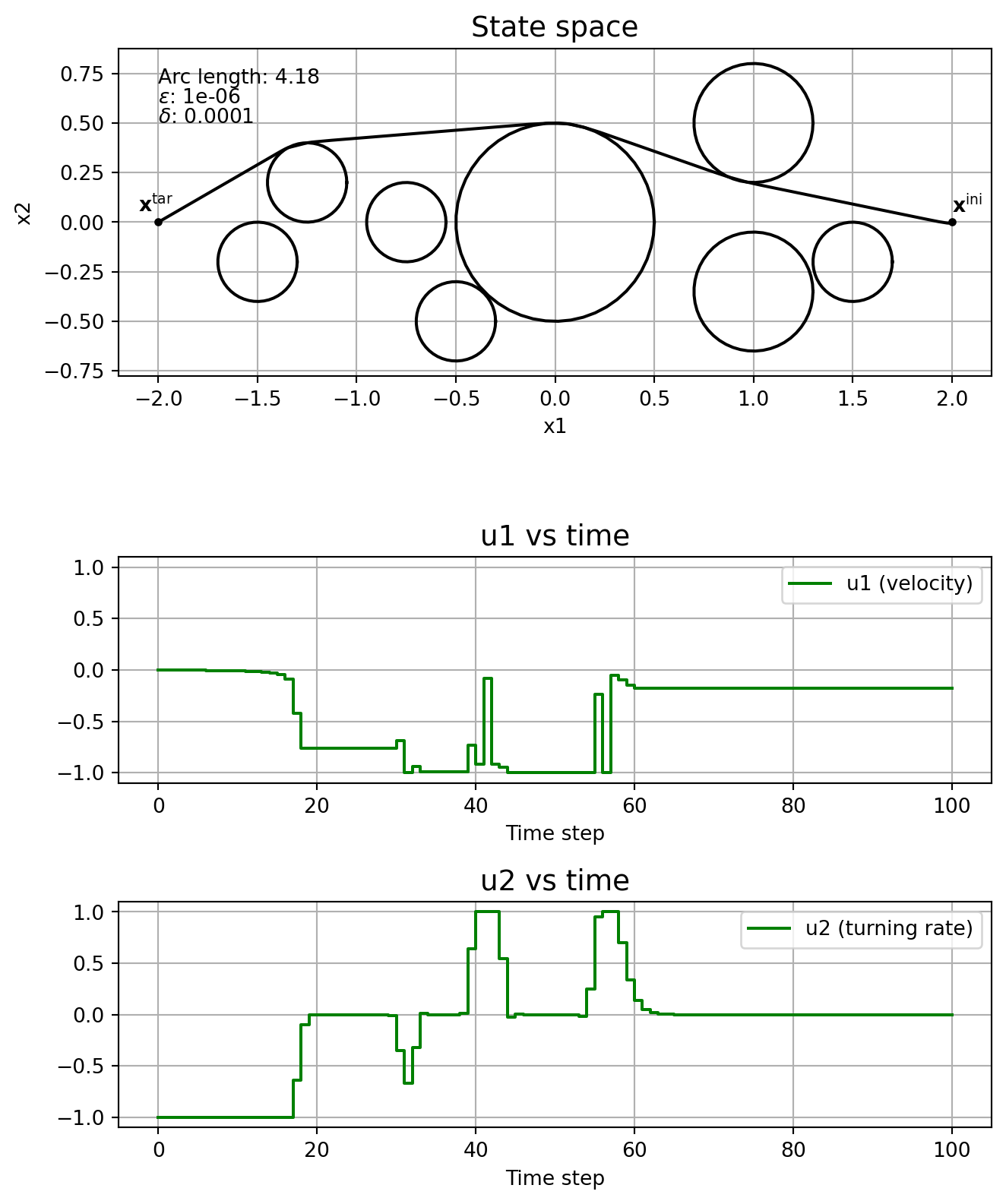
Figure 1: An example solution

1.1 Some notation

With \(\mathbf{x}(t)\in\mathbb{R}^n\) and \(t\in\mathbb{R}\), \(\dot{\mathbf{x}}(t) = \frac{\mathrm{d}}{\mathrm{d}t}\mathbf{x}(t)\) denotes the derivative of \(\mathbf{x}\) with respect to time, at time \(t\). With \(T\geq 0\), let \[\mathrm{PC}([0,T];\mathbb{R}^m) := \{f:[0,T] \rightarrow \mathbb{R}^m : f \text{ is continuous except at finitely many points in } [0,T]\},\] and \[\mathrm{C}([0,T];\mathbb{R}^n) := \{f:[0,T] \rightarrow \mathbb{R}^n : f \text{ is continuous on } [0,T]\}.\] For brevity, we’ll also use \(\mathrm{PC}_T^m := \mathrm{PC}([0,T];\mathbb{R}^m)\) and \(\mathrm{C}_T^n := \mathrm{C}([0,T];\mathbb{R}^n)\). The Euclidean norm of a vector \(\mathbf{x}\in\mathbb{R}^n\) is denoted by \(\Vert \mathbf{x}\Vert\). A Euclidean ball of radius \(\gamma>0\) about a point \(\mathbf{x}\in\mathbb{R}^n\) is denoted by \(\mathcal{B}_{\gamma}(\mathbf{x})\). With \(p,q\in\mathbb{Z}\) and \(0 \leq p \leq q\), the notation \([p:q] := \{p, p+1, \dots, q-1, q\}\) denotes all integers from \(p\) to \(q\). The notation \((\mathbb{R}^{n})^{N}\) denotes the set of all sequences of real \(n\)-dimensional vectors of length \(N\).

2 A car model

We’ll consider the following equations of motion, \[ \begin{align} \dot x_1(t) &= u_1(t)\cos(x_3(t)), \\ \dot x_2(t) &= u_1(t)\sin(x_3(t)), \\ \dot x_3(t) &= u_2(t), \end{align} \tag{1}\] where \(t \geq 0\) denotes time, \(x_1\in\mathbb{R}\) and \(x_2\in\mathbb{R}\) denote the car’s position, \(x_3\in\mathbb{R}\) denotes its orientation, \(u_1\in\mathbb{R}\) its velocity and \(u_2\in\mathbb{R}\) its rate of turning. This is a common model of a differential-drive robot, which consists of two wheels that can turn independently, see Figure 2. This allows it to drive forwards and backwards, rotate when stationary and perform other elaborate driving manoeuvres. Note that, because \(u_1\) can be \(0\), the model allows the car to stop instantaneously.

Figure 2: The differential drive robot, as modelled in (1).

Throughout the article we’ll let \(\mathbf{x}:= (x_1, x_2, x_3)^\top\in\mathbb{R}^3\) denote the state, \(\mathbf{u}:= (u_1, u_2)\in\mathbb{R}^2\) denote the control, and define \(f:\mathbb{R}^3\times\mathbb{R}^2 \rightarrow \mathbb{R}^3\) to be, \[ f(\mathbf{x},\mathbf{u}) := \left( \begin{array}{c} u_1\cos(x_3) \\ u_1\sin(x_3) \\ u_2 \end{array} \right), \] so that we can succinctly write the system as, \[ \dot{\mathbf{x}}(t) = f(\mathbf{x}(t), \mathbf{u}(t)),\quad t\geq 0. \tag{2}\]

3 Optimal path planning problem

Considering the car model in Section 2, we want to find the shortest path connecting an initial and target position while avoiding a number of obstacles. To that end, we’ll consider the following optimal control problem¹: \[ \mathrm{OCP}: \begin{cases} \min\limits_{\mathbf{x}, \mathbf{u}} \quad & J(\mathbf{x}, \mathbf{u})\\ \mathrm{subject\ to:}\quad & \dot{\mathbf{x}}(t) = f(\mathbf{x}(t),\mathbf{u}(t)), \quad & \mathrm{a.e.}\,\, t \in[0,T], & \\ \quad & \mathbf{x}(0) = \mathbf{x}^{\mathrm{ini}}, & & \\ \quad & \mathbf{x}(T) = \mathbf{x}^{\mathrm{tar}}, & & \\ \quad & \mathbf{u}(t) \in \mathbb{U}, \quad & \mathrm{a.e.}\,\, t \in[0,T], & \\ \quad & (x_1(t) - c_1^i)^2 + (x_2(t) - c_2^i)^2 \geq r_i^2, \quad & \forall t\in[0,T],\, \forall i\in \mathbb{I}, & \\ \quad & (\mathbf{x}, \mathbf{u}) \in \mathrm{C}_T^3\times\mathrm{PC}_T^2, \end{cases} \] where \(T\geq 0\) is the finite time horizon, \(J:\mathrm{C}_T^3\times\mathrm{PC}_T^2\rightarrow \mathbb{R}_{\geq 0}\) is the cost functional, \(\mathbf{x}^{\mathrm{ini}} \in\mathbb{R}^3\) is the initial state and \(\mathbf{x}^{\mathrm{tar}}\in\mathbb{R}^3\) is the target state. The control is constrained to \(\mathbb{U}:= [\underline{u}_1, \overline{u}_1]\times [\underline{u}_2, \overline{u}_2]\), with \(\underline{u}_j < 0 <\overline{u}_j\), \(j=1,2\). Circular obstacles are given by a centre, \((c_1^i, c_2^i)\in\mathbb{R}^2\), and a radius, \(r_i\in\mathbb{R}_{\geq 0}\), with \(\mathbb{I}\) indicating the indices of all obstacles. For the cost functional we’ll consider the arc length of the curve connecting \(\mathbf{x}^{\mathrm{ini}}\) and \(\mathbf{x}^{\mathrm{tar}}\), that is, \[ J(\mathbf{x},\mathbf{u}) = \int_0^T\left(\sqrt{\dot x_1^2(s) + \dot x_2^2(s)}\right)\, \mathrm{d}s. \]

3.1 Some comments on the OCP

The equations of motion and the presence of obstacles make the optimal control problem nonlinear and nonconvex, which is difficult to solve in general. A solver may converge to locally optimal solutions, which are not necessarily globally optimal, or it may fail to find a feasible solution even though one exists.

For simplicity the obstacles are circles. These are nice because they’re differentiable, so we can use a gradient-based algorithm to solve the OCP. (We’ll use IPOPT, which implements an interior-point method.)

The arc length function, \(J\), is not differentiable when the car’s speed is zero. However, as we’ll see, we can eliminate this problem by adding a small \(\varepsilon > 0\) under the square-root.

Depending on the scheme used to discretise the equations of motion, there may be chattering in the control signal. As we’ll see, this can easily be dealt with by penalising excessive control action in the cost function.

The horizon length considered in the problem, \(T\), is fixed. Thus, as the problem is posed, we actually want to find the curve of shortest arc length for which the car reaches the target in exactly \(T\) seconds. This is actually not an issue for our car because it can stop instantaneously and rotate on the spot. So, the solutions to the OCP (if the solver can find them) might consist of long boring chunks at the beginning and/or end of the time period if \(T\) is very large. If we wanted to make the horizon length a decision variable in the problem then we have two options. First, if we use a direct method to numerically solve the problem (as we will do in the next section) we could vary the horizon length by making the discretisation step size appearing in the numerical integration a decision variable. This is because the dimension of the decision space must be set at the time at which you invoke the numerical nonlinear programme solver. The second option is to resort to an indirect method (in a nutshell, you need to solve a boundary-value problem that you get from an analysis of the problem via Pontryagin’s principle, often via the shooting method). However, for a problem like ours, where you have many state constraints, this can be quite difficult.

4 Deriving a sensible nonlinear programme

We’ll solve the optimal control problem using direct single shooting. More precisely, we’ll take the control to be piecewise constant over a uniform grid of time intervals and propagate the state trajectory from the initial condition using the fourth-order Runge-Kutta (RK4) method. We’ll then form a finite-dimensional nonlinear programme (NLP), where the decision variables consist of the state and control at each discrete time step. This section shows how to form a “sensible” NLP, which deals with the various numerical difficulties.

4.1 The RK4 scheme

Consider the car’s differential equation, Equation (2), with initial condition, \(\mathbf{x}^{\mathrm{ini}}\), over an interval, \([0,T]\), \[ \dot{\mathbf{x}}(t) = f(\mathbf{x}(t), \mathbf{u}(t)), \quad t\in[0,T], \quad \mathbf{x}(0) = \mathbf{x}^{\mathrm{ini}}. \] Let \(h>0\) denote the constant time step, and let \(K := \mathrm{floor}(T/h)\). Then the RK4 scheme reads, \[ \mathbf{x}[k+1] = \mathbf{x}[k] + \frac{h}{6}\mathrm{RK}_4(\mathbf{x}[k], \mathbf{u}[k]), \quad \forall \,\, k \in[0:K-1], \quad \mathbf{x}[0] = \mathbf{x}(0), \] where \(\mathrm{RK}_4:\mathbb{R}^3\times \mathbb{R}^2 \rightarrow \mathbb{R}^3\) reads, \[ \mathrm{RK}_4(\mathbf{x}, \mathbf{u}) = k_1 + 2k_2 + 2k_3 + k_4, \] and \[ k_1 = f(\mathbf{x}, \mathbf{u}),\quad k_2 = f(\mathbf{x}+ \frac{h}{2}k_1, \mathbf{u}), \quad k_3 = f(\mathbf{x}+ \frac{h}{2}k_2, \mathbf{u}),\quad k_4 = f(\mathbf{x}+ hk_3, \mathbf{u}). \] The notation \(\mathbf{x}[k]\) and \(\mathbf{u}[k]\) is meant to denote the discretised state and control, respectively, so as to distinguish them from their continuous-time counterparts.

4.2 Singularity of the cost functional

You might be tempted to consider the polygonal arc length as the cost in the NLP, namely, \[ \sum_{k=0}^{K-1}\Vert\mathbf{x}[k+1] - \mathbf{x}[k]\Vert = \sum_{k=0}^{K-1}\sqrt{(x_{1}[k+1] - x_1[k])^2 + (x_2[k+1] - x_2[k])^2}. \] However, this function is not differentiable if for some \(k\in\{0,1,\dots,K-1\}\), \[ \Vert\mathbf{x}[k+1] - \mathbf{x}[k]\Vert = 0, \] which often leads to the solver failing. You might see the error EXIT: Invalid number in NLP function or derivative detected if you solve a problem with this article’s code (which uses IPOPT, a gradient-based solver).

One solution is to approximate the polygonal arc length with, \[ \sum_{k=0}^{K-1}\sqrt{(x_{1}[k+1] - x_1[k])^2 + (x_2[k+1] - x_2[k])^2 + \varepsilon}, \] with \(\varepsilon > 0\) a small number. We see that, for an arbitrary \(k\in\{1,\dots,K-1\}\) and \(i\in\{1,2\}\), \[ \begin{align*} \frac{\partial}{\partial x_i[k]} &\left( \sum_{m=0}^{K-1} \sqrt{(x_1[m+1] - x_1[m])^2 + (x_2[m+1] - x_2[m])^2 + \varepsilon} \right) \\[6pt] &= \frac{x_i[k] - x_i[k-1]}{\sqrt{(x_1[k] - x_1[k-1])^2 + (x_2[k] - x_2[k-1])^2 + \varepsilon}} \\ &\quad + \frac{x_i[k] - x_i[k+1]}{\sqrt{(x_1[k+1] - x_1[k])^2 + (x_2[k+1] - x_2[k])^2 + \varepsilon}} \end{align*} \] and so this function is continuously differentiable, ensuring smooth gradients for IPOPT. (You get similar expressions if you look at \(\frac{\partial}{\partial x_i[K]}\) and \(\frac{\partial}{\partial x_i[0]}\)).

4.3 Control chattering

Control chattering is the rapid jumping/oscillation/switching of the optimal control signal. There may be parts of the solution that truly chatter (this may occur when the optimal control is bang-bang, for example) or a numerical solver may find a solution that chatters artificially. Delving into this deep topic is out of this article’s scope but, very briefly, you might encounter this phenomenon in problems where the optimal solution exhibits so-called active arcs. These are portions of the solution along which the state constraints are active, which, in our setting, corresponds to the car travelling along the boundaries of the obstacles along its optimal path. When solving problems exhibiting such arcs via a direct method, as we are doing, the numerical solver may approximate the true solution along these arcs with rapid oscillation.

Thankfully, a simple way to get rid of chattering is to just penalise control action by adding the term: \[ \delta\sum_{k=0}^{K-1}\Vert \mathbf{u}[k] \Vert^2 \] in the cost function, for some small \(\delta\). (This at least works well for our problem, even for very small \(\delta\).)

4.4 Scaling for good numerical conditioning

A well-scaled nonlinear programme is one where small changes in the decision variable result in small changes in the cost and the values of the constraint functions (the so-called constraint residuals). We can check how well our problem is scaled by looking at the magnitude of the cost function, at its gradient and Hessian, as well the Jacobian of the constraint function at points in the decision space (in particuar, at the initial warm start and points close to the solution). If these quantities are of comparable order then the solver will be robust, meaning it will usually converge in relatively few steps. A badly-scaled problem may take extremely long to converge (because it might need to take very small steps of the decision variable) or simply fail.

Considering our problem, it makes sense to scale the cost by roughly the length we expect the final path to be. A good choice is the length of the line connecting the initial and target positions, call this \(L\). Moreover, it then makes sense to scale the constraints by \(1/L^2\) (because we are squaring quantities here).

4.5 The sensible nonlinear programme

Taking the discussions of the previous subsections into account, the sensible NLP that we’ll consider in the numerics section reads, \[ \mathrm{NLP}_{\varepsilon, \delta}: \begin{cases} \min\limits_{\mathbf{x}, \mathbf{u}} \quad & J_{\varepsilon,\delta}(\mathbf{x}, \mathbf{u}) \\ \mathrm{subject\ to:} \quad & \mathbf{x}[k+1] = \mathbf{x}[k] + \frac{h}{6}\mathrm{RK}_4(\mathbf{x}[k], \mathbf{u}[k]), & \forall k \in[0:K-1], &\\ \quad & \mathbf{x}[0] = \mathbf{x}^{\mathrm{ini}}, & \\ \quad & \mathbf{x}[K] = \mathbf{x}^{\mathrm{tar}}, & \\ \quad & \mathbf{u}[k]\in \mathbb{U}, & \forall k \in[0:K-1], & \\ \quad & \frac{1}{L^2}\left( x_1[k] - c_1^i \right)^2 + \frac{1}{L^2}\left( x_2[k] - c_2^i \right)^2 \geq \frac{1}{L^2} r_i^2, \quad & \forall k \in[0:K], & \forall i\in \mathbb{I},\\ \quad & (\mathbf{x}, \mathbf{u}) \in (\mathbb{R}^{3})^K \times (\mathbb{R}^{2})^{K-1}, & \end{cases} \] where \(J_{\varepsilon,\delta}: (\mathbb{R}^{3})^K \times (\mathbb{R}^{2})^{K-1} \rightarrow \mathbb{R}_{>0}\) is defined to be, \[ J_{\varepsilon,\delta}(\mathbf{x}, \mathbf{u}) := \frac{1}{L} \left(\sum_{k=0}^{K-1}\sqrt{\Vert \mathbf{x}[k+1] - \mathbf{x}[k]\Vert^2 + \varepsilon } + \delta\sum_{k=0}^{K-1}\Vert \mathbf{u}[k] \Vert^2 \right). \]

To aid upcoming discussion, define the feasible set, \(\Omega\), to be the set of all pairs \((\mathbf{x},\mathbf{u})\) that satisfy the constraints of \(\mathrm{NLP}_{\varepsilon, \delta}\). A feasible pair \((\mathbf{x}^{(\varepsilon,\delta)}, \mathbf{u}^{(\varepsilon,\delta)})\) is said to be globally optimal provided that, \[ J_{\varepsilon,\delta}(\mathbf{x}^{(\varepsilon,\delta)}, \mathbf{u}^{(\varepsilon,\delta)}) \leq J_{\varepsilon,\delta}(\mathbf{x}, \mathbf{u}),\quad\forall(\mathbf{x}, \mathbf{u}) \in \Omega. \] A feasible pair \((\mathbf{x}^{(\varepsilon,\delta)}, \mathbf{u}^{(\varepsilon,\delta)})\) is said to be locally optimal provided that there exists a small enough \(\gamma >0\) for which, \[ J_{\varepsilon,\delta}(\mathbf{x}^{(\varepsilon,\delta)}, \mathbf{u}^{(\varepsilon,\delta)}) \leq J_{\varepsilon,\delta}(\mathbf{x}, \mathbf{u}),\quad\forall(\mathbf{x}, \mathbf{u}) \in \Omega\cap \mathcal{B}_{\gamma}(\mathbf{x}^{(\varepsilon,\delta)}, \mathbf{u}^{(\varepsilon,\delta)}). \]

5 A homotopy method

Recall that the problem is nonlinear and nonconvex. Thus, if we were to just choose a small \(\varepsilon>0\) and \(\delta>0\) and throw \(\mathrm{NLP}_{\varepsilon, \delta}\) at a solver, then it could fail even though feasible pairs might exist, or it may find “bad” locally optimal pairs.

One approach to deal with these issues is to guide the solver towards a solution by successively solving easier problems that converge to the difficult problem. This is the idea behind using a homotopy method². We will guide the solver towards a solution with a simple algorithm that successively gives the solver a good warm start:

Homotopy algorithm

Input: Initial parameters \(\varepsilon_{\mathrm{ini}}>0\), \(\delta_{\mathrm{ini}}>0\). Tolerances \(\mathrm{tol}_{\varepsilon}>0\), \(\mathrm{tol}_{\delta}>0\).

Output: Solution \((\mathbf{x}^{(\mathrm{tol}_{\varepsilon}, \mathrm{tol}_{\delta})}, \mathbf{u}^{(\mathrm{tol}_{\varepsilon}, \mathrm{tol}_{\delta})})\) (if it can find one)

1. Get initial warm start, \((\mathbf{x}^{\mathrm{warm}}, \mathbf{u}^{\mathrm{warm}})\) (not necessarily feasible)
2. \(i \gets 0\)
3. While \(\varepsilon > \mathrm{tol}_{\varepsilon}\) and \(\delta > \mathrm{tol}_{\delta}\):
   • \(\varepsilon\gets \max \{ \varepsilon_{\mathrm{ini}} / 2^i, \mathrm{tol}_{\varepsilon} \}\)
   • \(\delta\gets \max \{ \delta_{\mathrm{ini}} / 2^i, \mathrm{tol}_{\delta} \}\)
   • Solve \(\mathrm{NLP}_{\varepsilon, \delta}\) with warm start \((\mathbf{x}^{\mathrm{warm}}, \mathbf{u}^{\mathrm{warm}})\).
   • Label the solution \((\mathbf{x}^{(\varepsilon, \delta)}, \mathbf{u}^{(\varepsilon, \delta)})\).
   • \((\mathbf{x}^{\mathrm{warm}}, \mathbf{u}^{\mathrm{warm}})\gets (\mathbf{x}^{(\varepsilon, \delta)}, \mathbf{u}^{(\varepsilon, \delta)})\)
   • \(i\gets i + 1\)
4. Return \((\mathbf{x}^{(\mathrm{tol}_{\varepsilon}, \mathrm{tol}_{\delta})}, \mathbf{u}^{(\mathrm{tol}_{\varepsilon}, \mathrm{tol}_{\delta})})\)

Important

The homotopy algorithm is meant to help the solver find a good solution. Note however, that there is no guarantee that it will successfully find even a feasible solution, nevermind a globally optimal one. For some theory regarding so-called globally convergent homotopies you can consult the papers, Watson (2001) and Esterhuizen et al. (2025).

6 Numerical experiments

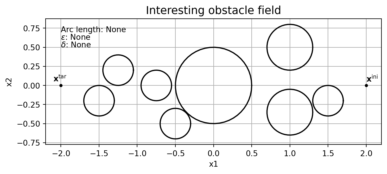
In this section we’ll consider \(\mathrm{NLP}_{\varepsilon, \delta}\) with initial and target states \(\mathbf{x}^{\mathrm{ini}} = (2,0,\frac{\pi}{2})\) and \(\mathbf{x}^{\mathrm{tar}} = (-2,0,\mathrm{free})\), respectively (thus \(L = 4\)). We’ll take the horizon as \(T=10\) and keep the discretisation step size in the RK4 scheme constant at \(h=0.1\), thus \(K=100\). As the control constraints we’ll take \(\mathbb{U} = [-1,1] \times [-1, 1]\), and we’ll consider this interesting obstacle field:

from car_OCP import plot_solution_in_state_space
x_tot = [[2,-2],[0,0]]

obstacles = [
    {'centre': (0,0), 'radius': 0.5},
    {'centre': (-0.5,-0.5), 'radius': 0.2},
    {'centre': (1,0.5), 'radius': 0.3},
    {'centre': (1,-0.35), 'radius': 0.3},
    {'centre': (-1.5,-0.2), 'radius': 0.2},
    {'centre': (1.5,-0.2), 'radius': 0.2},
    {'centre': (-0.75,0), 'radius': 0.2},
    {'centre': (-1.25,0.2), 'radius': 0.2}
]

plot_solution_in_state_space(x_tot, obstacles, 'Interesting obstacle field', arc_length=None, obstacles_only=True)

6.1 Checking conditioning

First, we’ll check the problem’s scaling at the warm start. Stack the state and control into a long vector, \(\mathbf{d}\in\mathbb{R}^{3K + 2(K-1)}\), as follows: \[\mathbf{d} := (x_1[0],x_2[0],x_3[0],x_1[1],x_2[1],x_3[1],\dots,u_1[0],u_2[0],u_1[1],u_2[1],\dots,u_1[K-1],u_2[K-1]),\] and write \(\mathrm{NLP}_{\varepsilon, \delta}\) as: \[ \begin{cases} \min\limits_{\mathbf{d}} \quad & J_{\varepsilon,\delta}(\mathbf{d}) \\ \mathrm{subject\ to:} \quad & g(\mathbf{d}) \leq \mathbf{0}, \end{cases} \] where \(g\) collects all the constraints. As a warm start, call this vector \(\mathbf{d}^{\mathrm{ini}}\), we’ll take the line connecting the initial and target positions, with \(u_1[k] \equiv 0.1\) and \(u_2[k] \equiv 0\). We should have a look at the magnitudes of the following quantities at the point \(\mathbf{d}^{\mathrm{ini}}\):

• The cost function, \(J_{\varepsilon,\delta}(\mathbf{d}^{\mathrm{ini}})\)
• Its gradient, \(\nabla J_{\varepsilon,\delta}(\mathbf{d}^{\mathrm{ini}})\)
• Its Hessian, \(\mathbf{H}(J_{\varepsilon,\delta}(\mathbf{d}^{\mathrm{ini}}))\)
• The constraint residual, \(g(\mathbf{d}^{\mathrm{ini}})\)
• Its Jacobian, \(\mathbf{J}(g(\mathbf{d}^{\mathrm{ini}}))\)

We can do this with the code from the repo:

import numpy as np
from car_OCP import get_initial_warm_start, build_and_check_scaling

x_init = np.array([[2],[0],[np.pi/2]])
x_target = np.array([[-2],[0]])

T = 10 # Horizon length
h = 0.1 # RK4 time step

obstacles = [
    {'centre': (0,0), 'radius': 0.5},
    {'centre': (-0.5,-0.5), 'radius': 0.2},
    {'centre': (1,0.5), 'radius': 0.3},
    {'centre': (1,-0.35), 'radius': 0.3},
    {'centre': (-1.5,-0.2), 'radius': 0.2},
    {'centre': (1.5,-0.2), 'radius': 0.2},
    {'centre': (-0.75,0), 'radius': 0.2},
    {'centre': (-1.25,0.2), 'radius': 0.2}
]

constraints = {
    'u1_min' : -1,
    'u1_max' : 1,
    'u2_min' : -1,
    'u2_max' : 1,
}

warm_start = get_initial_warm_start(x_init, x_target, T, h)

build_and_check_scaling(x_init, x_target, obstacles, constraints, T, h, warm_start, eps=1e-4, delta=1e-4)

=== SCALING DIAGNOSTICS ===
Objective J          : 1.031e+00
||∇J||_2             : 3.430e-01
||Hess J||_Frob      : 1.485e+02
||g||_2              : 7.367e+00
||Jac g||_Frob       : 2.896e+01
============================

With small \(\varepsilon\) and \(\delta\), and with our chosen \(\mathbf{d}^{\mathrm{ini}}\), the objective should obviously be close to 1. The size of its gradient and of the constraint residuals at the warm start should be of similar order. In the print-out, \(\Vert \nabla J \Vert_2\) denotes the Euclidean norm. The cost function’s Hessian can be of larger order (this increases with a finer time step). In the print-out, \(\Vert \nabla \mathrm{Hess} \ J \Vert_{\mathrm{Frob}}\) is the Frobenius norm of the Hessian matrix, which, intuitively speaking, tells you “how big” the linear transformation is “on average”, so it’s a good measure to consider. The Jacobian of \(g\) can also be of slightly larger order.

The print-out shows that our problem is well-scaled, great. But one last thing we’ll also do is tell IPOPT to scale the problem before we solve it, with "ipopt.nlp_scaling_method":

.... set up problem ....

opts = {"ipopt.print_level": 0, 
        "print_time": 0, 
        "ipopt.sb": "yes",
        "ipopt.nlp_scaling_method": "gradient-based"}

opti.minimize(cost)
opti.solver("ipopt", opts)

6.2 Solving WITHOUT homotopy

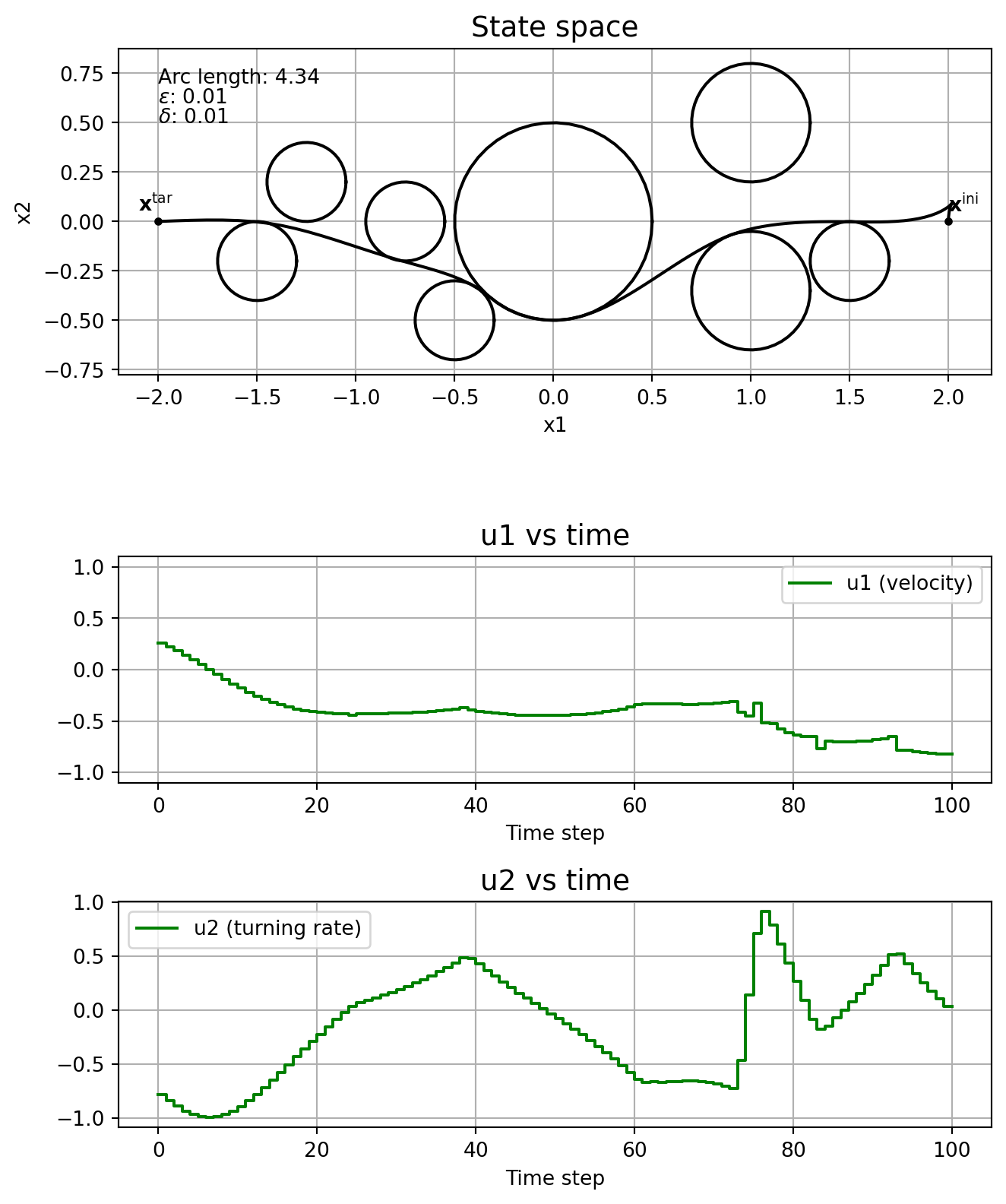
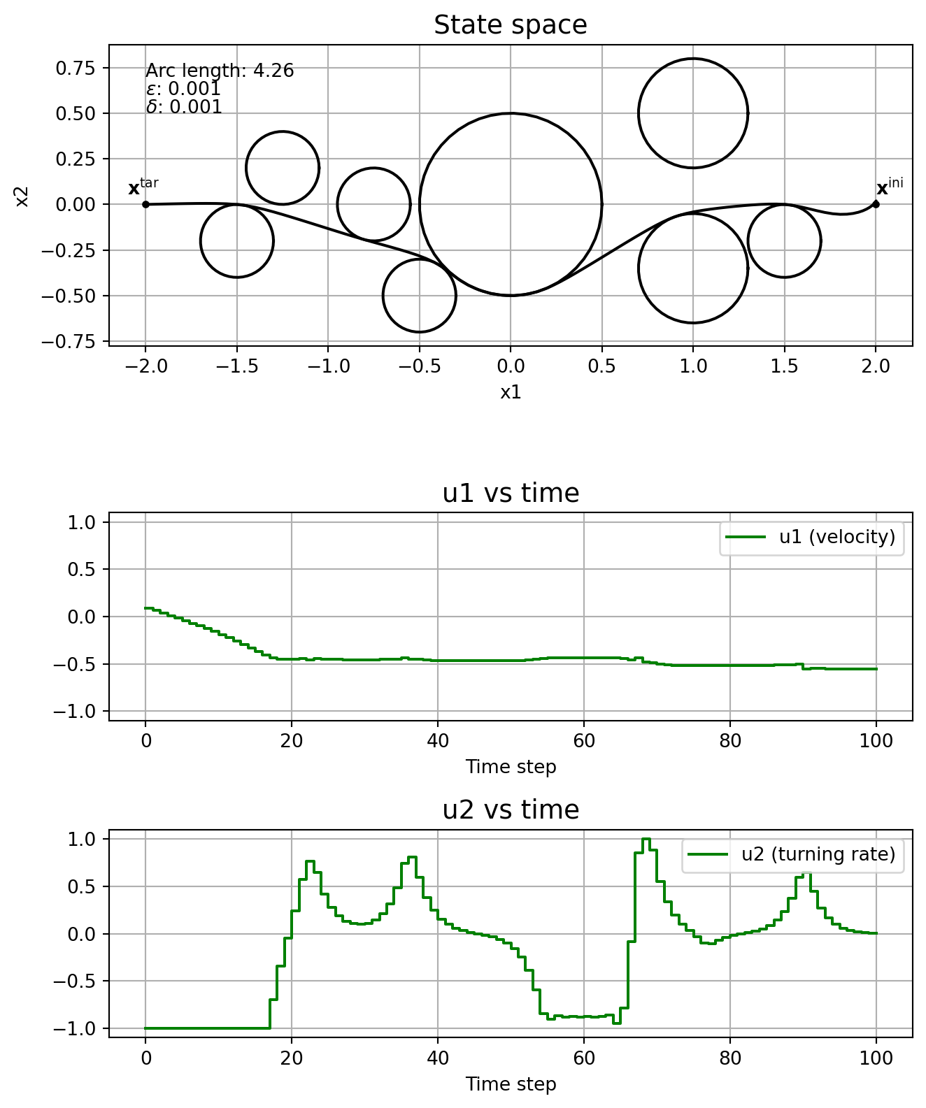
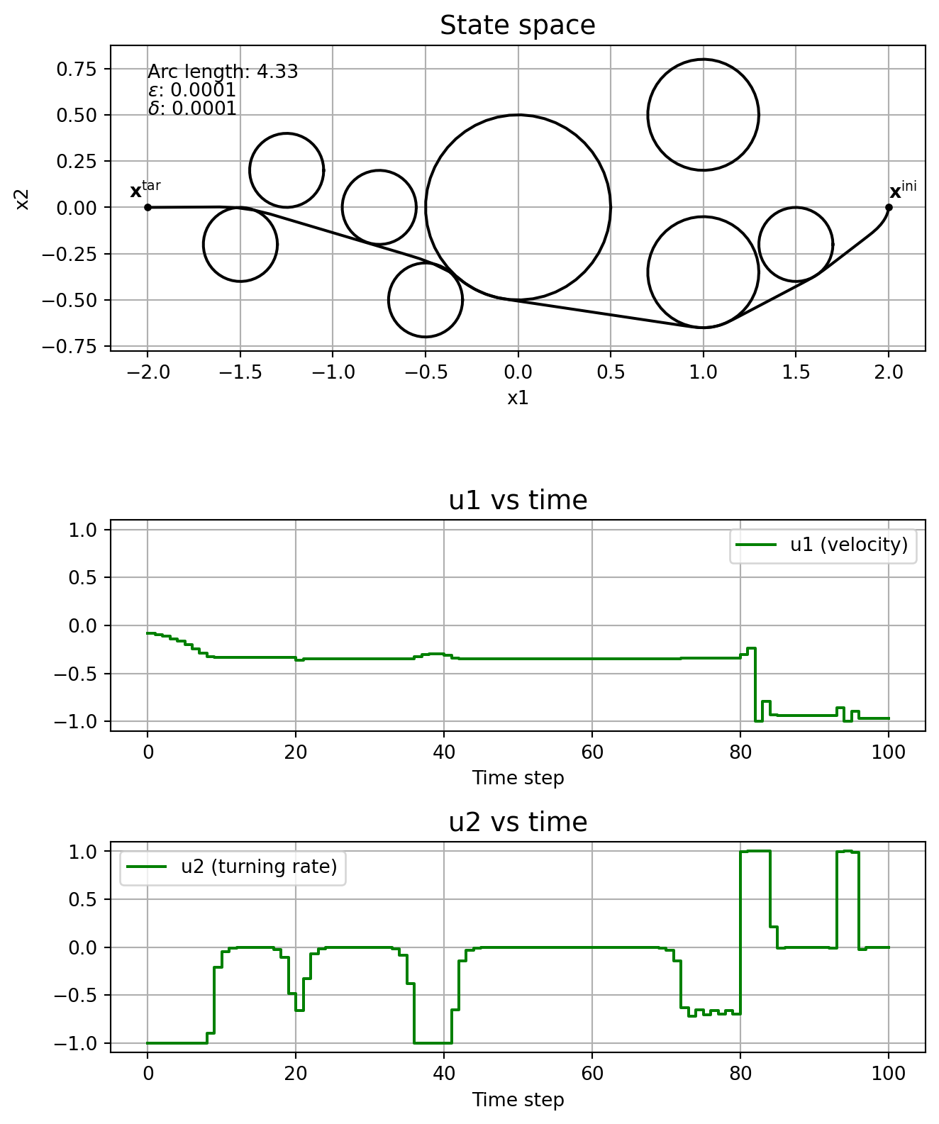
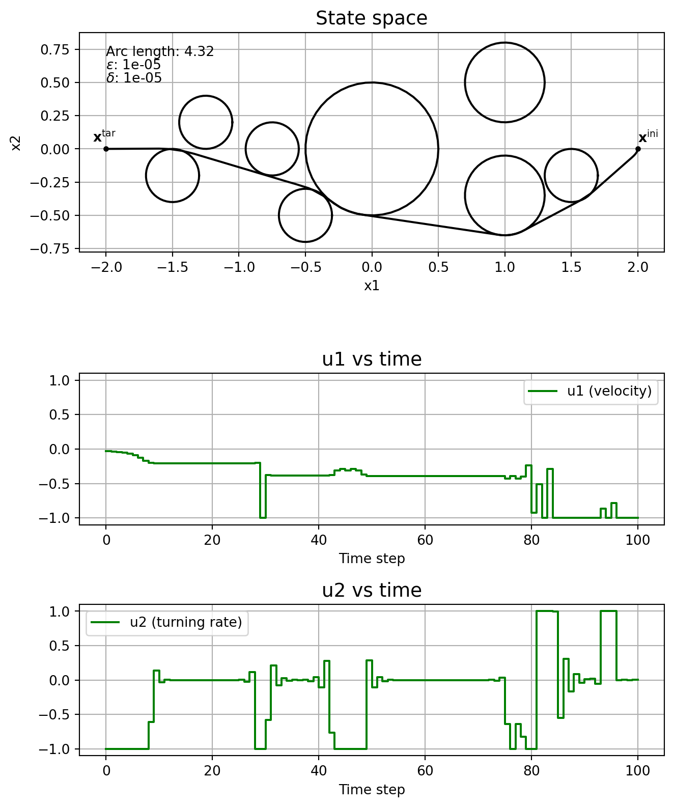
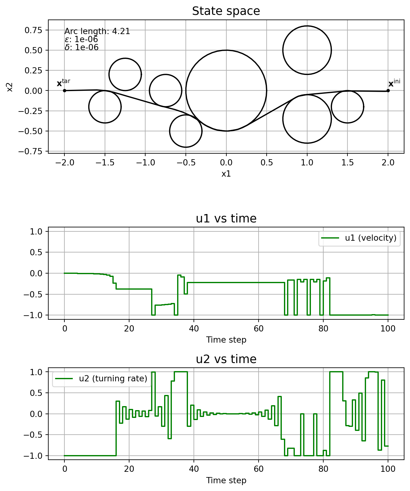
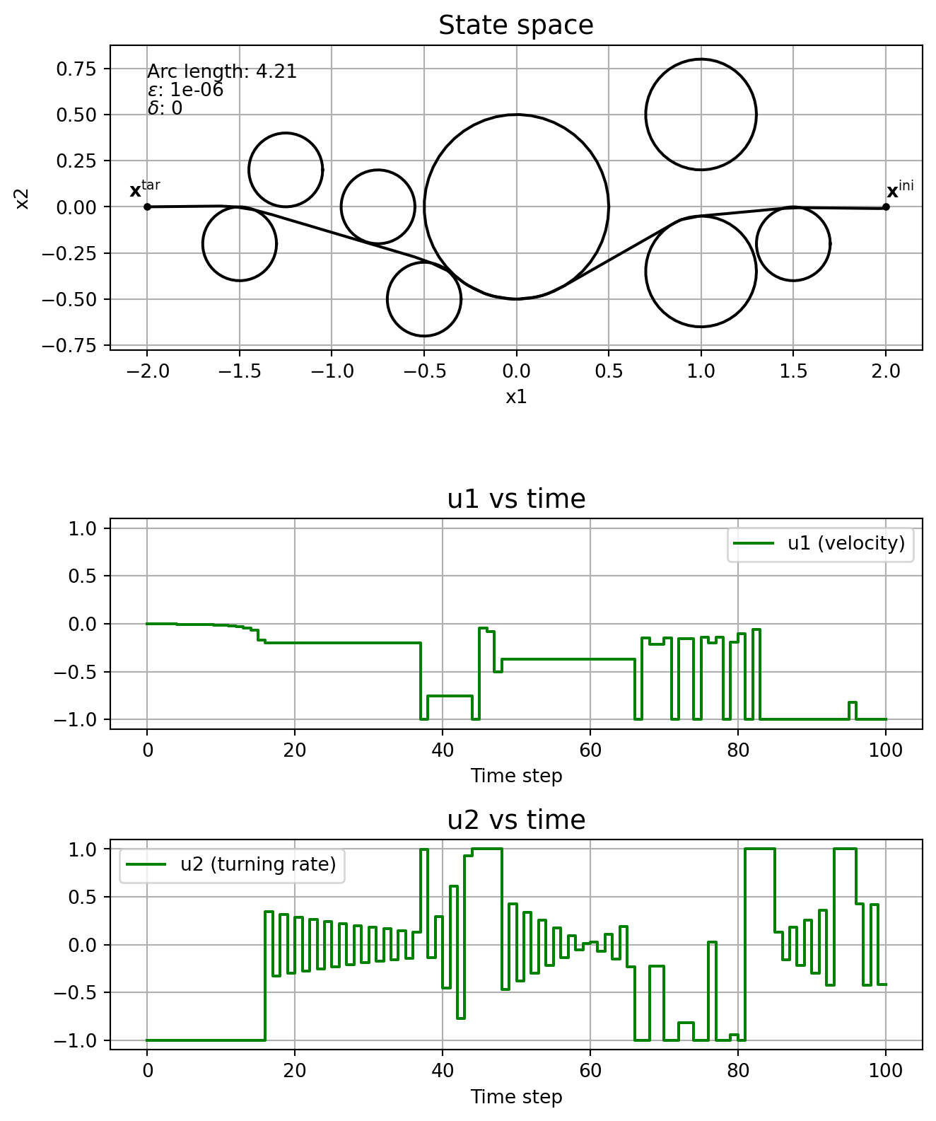
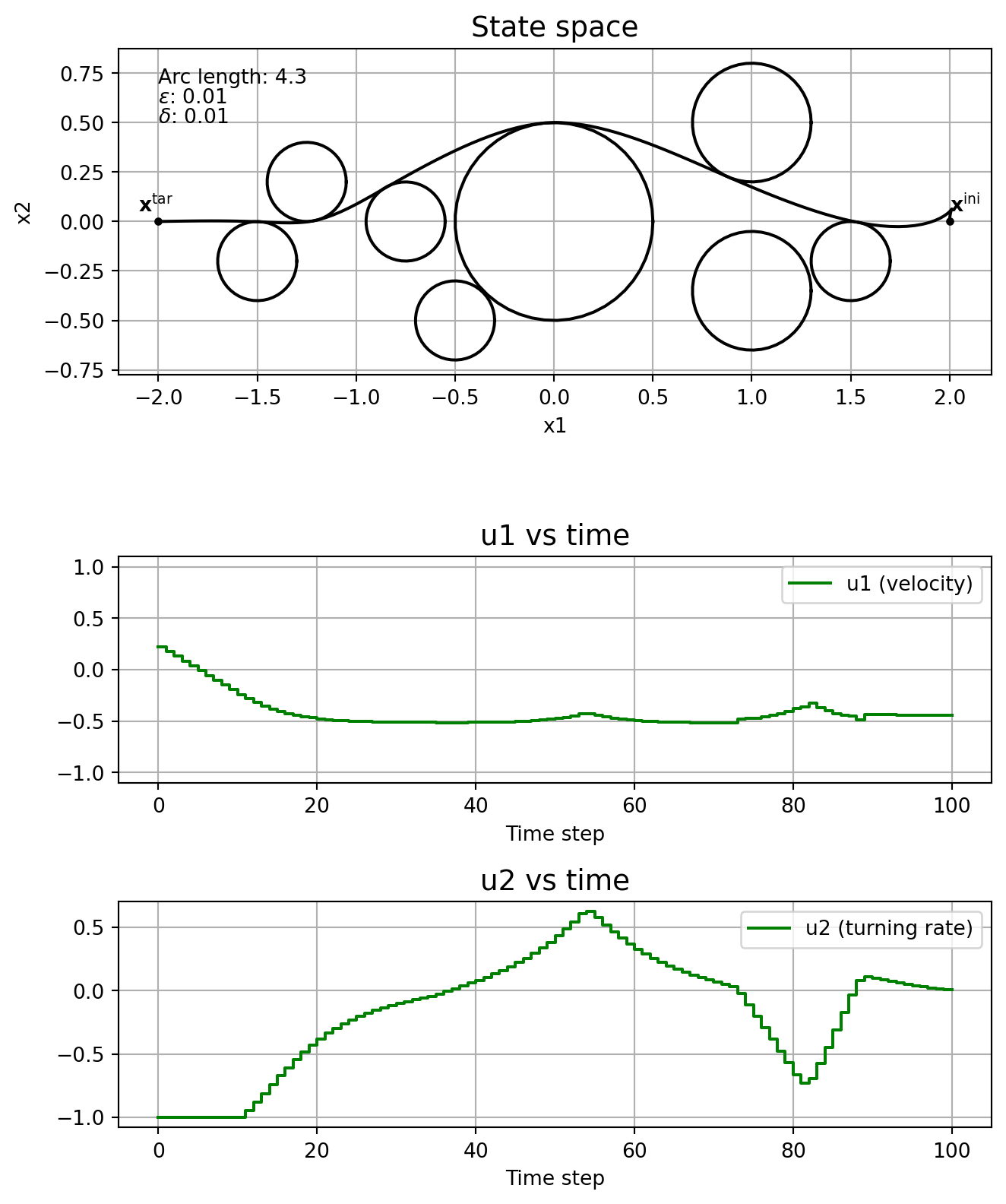
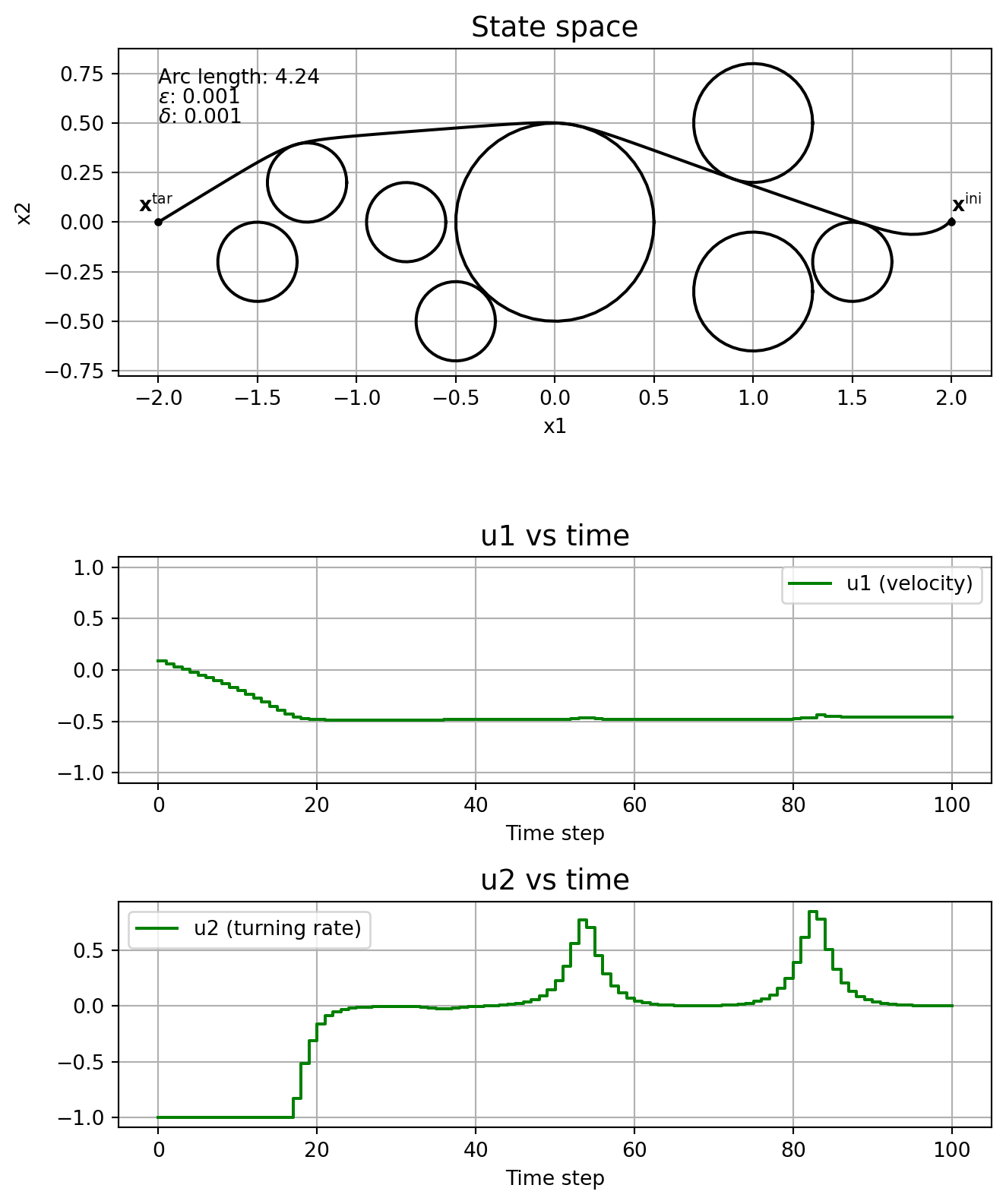
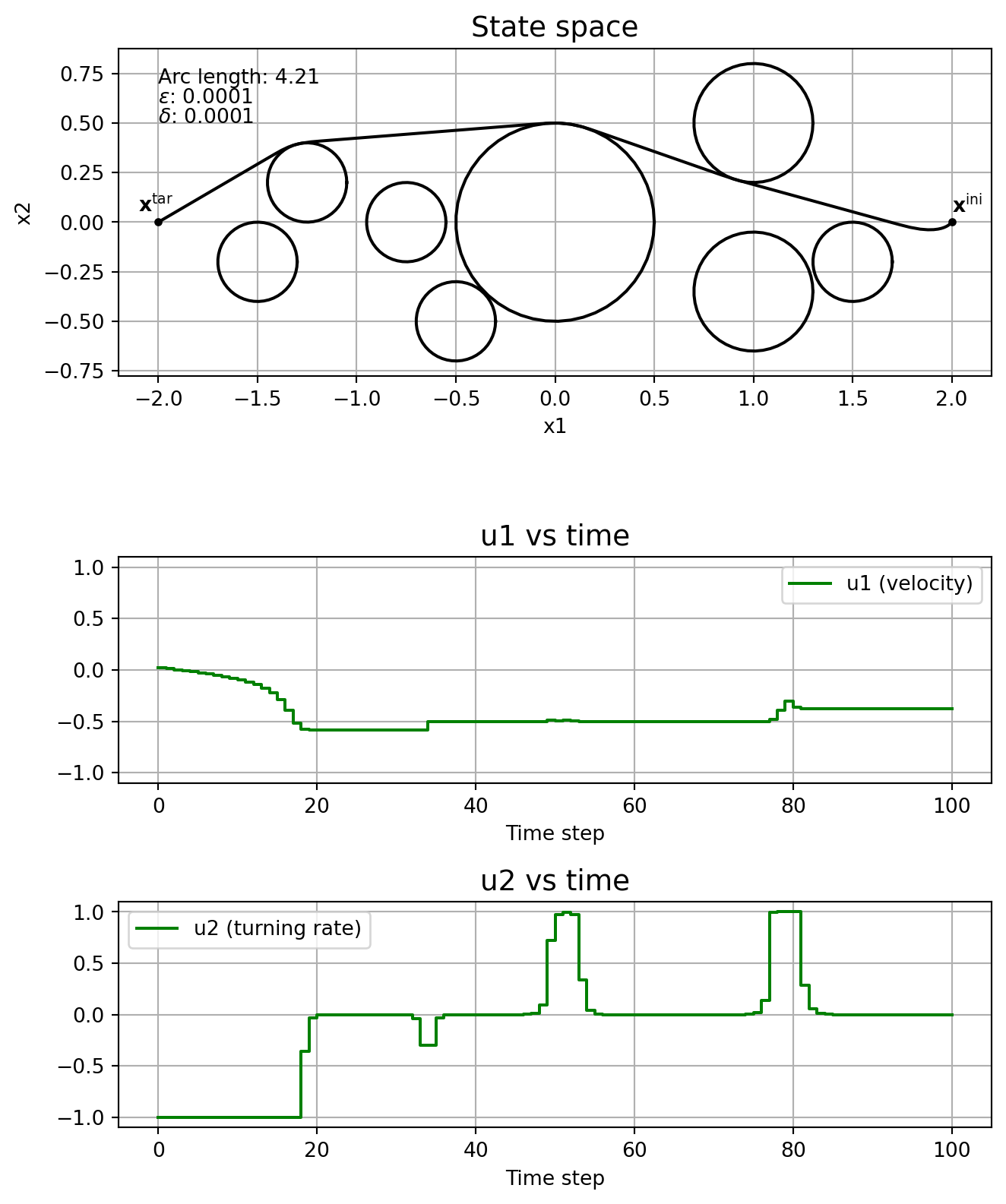
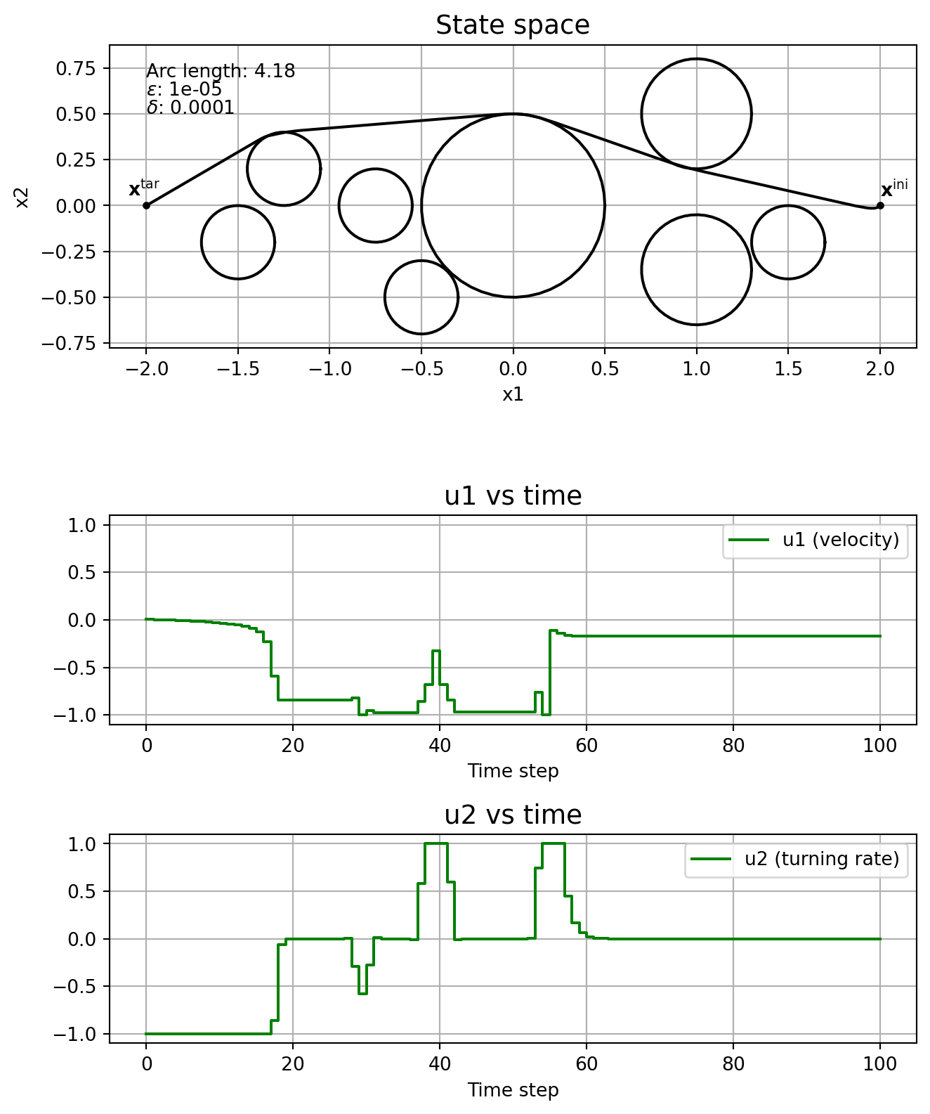
This subsection shows the effect of the parameters \(\varepsilon\) and \(\delta\) on the solution, without running the homotopy algorithm. In other words, we fix \(\varepsilon\) and \(\delta\), and solve \(\mathrm{NLP}_{\varepsilon, \delta}\) straight, without even specifying a good initial guess.

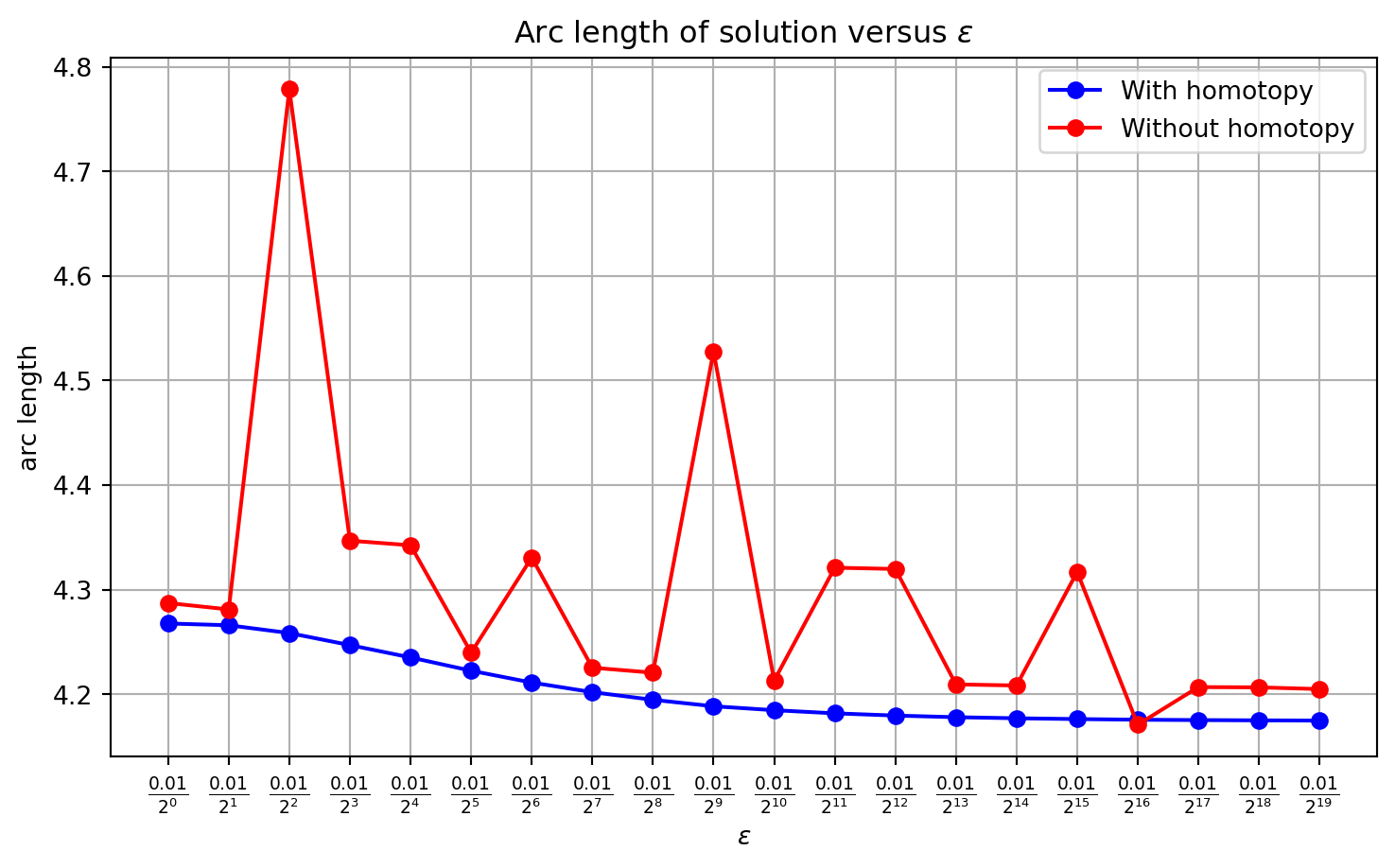
Note how the solver might find locally optimal solutions that are clearly not so good, like in the cases \(\varepsilon\) = \(\delta\) = 1e-4, and \(\varepsilon\) = \(\delta\) = 1e-5. This is one motivation for using homotopy: you could guide the solver to a better locally optimal solution. Note how \(\delta\) affects the chattering, with it being really bad when \(\delta=0\). The solver just fails when \(\varepsilon=0\).

\(\varepsilon=\delta\) = 1e-2

import numpy as np
from car_OCP import solve_OCP, get_arc_length, plot_solution_in_statespace_and_control

eps=1e-2
delta=1e-2

x_init = np.array([[2],[0],[np.pi/2]])
x_target = np.array([[-2],[0]])

T = 10 # Horizon length
h = 0.1 # RK4 time step

obstacles = [
    {'centre': (0,0), 'radius': 0.5},
    {'centre': (-0.5,-0.5), 'radius': 0.2},
    {'centre': (1,0.5), 'radius': 0.3},
    {'centre': (1,-0.35), 'radius': 0.3},
    {'centre': (-1.5,-0.2), 'radius': 0.2},
    {'centre': (1.5,-0.2), 'radius': 0.2},
    {'centre': (-0.75,0), 'radius': 0.2},
    {'centre': (-1.25,0.2), 'radius': 0.2}
]

constraints = {
    'u1_min' : -1,
    'u1_max' : 1,
    'u2_min' : -1,
    'u2_max' : 1,
}

x_opt, u_opt = solve_OCP(x_init, x_target, obstacles, constraints, T, h, warm_start=None, eps=eps, delta=delta)

plot_solution_in_statespace_and_control(x_opt, u_opt, obstacles, arc_length=np.round(get_arc_length(x_opt), 2), obstacles_only=False, eps=eps, delta=delta)

\(\varepsilon=\delta\) = 1e-3

eps=1e-3
delta=1e-3

x_opt, u_opt = solve_OCP(x_init, x_target, obstacles, constraints, T, h, warm_start=None, eps=eps, delta=delta)

plot_solution_in_statespace_and_control(x_opt, u_opt, obstacles, arc_length=np.round(get_arc_length(x_opt), 2), obstacles_only=False, eps=eps, delta=delta)

\(\varepsilon=\delta\) = 1e-4

eps=1e-4
delta=1e-4

x_opt, u_opt = solve_OCP(x_init, x_target, obstacles, constraints, T, h, warm_start=None, eps=eps, delta=delta)

plot_solution_in_statespace_and_control(x_opt, u_opt, obstacles, arc_length=np.round(get_arc_length(x_opt), 2), obstacles_only=False, eps=eps, delta=delta)

\(\varepsilon=\delta\) = 1e-5

eps=1e-5
delta=1e-5

x_opt, u_opt = solve_OCP(x_init, x_target, obstacles, constraints, T, h, warm_start=None, eps=eps, delta=delta)

plot_solution_in_statespace_and_control(x_opt, u_opt, obstacles, arc_length=np.round(get_arc_length(x_opt), 2), obstacles_only=False, eps=eps, delta=delta)

\(\varepsilon=\delta\) = 1e-6

eps=1e-6
delta=1e-6

x_opt, u_opt = solve_OCP(x_init, x_target, obstacles, constraints, T, h, warm_start=None, eps=eps, delta=delta)

plot_solution_in_statespace_and_control(x_opt, u_opt, obstacles, arc_length=np.round(get_arc_length(x_opt), 2), obstacles_only=False, eps=eps, delta=delta)

\(\varepsilon\) = 1e-6, \(\delta\) = 0

eps=1e-6
delta=0

try:
  x_opt, u_opt = solve_OCP(x_init, x_target, obstacles, constraints, T, h, warm_start=None, eps=eps, delta=delta)

  plot_solution_in_statespace_and_control(x_opt, u_opt, obstacles, arc_length=np.round(get_arc_length(x_opt), 2), obstacles_only=False, eps=eps, delta=delta)

except Exception as error:
  print(f'Error: {error}')

\(\varepsilon=\delta\) = 0

eps=0
delta=0

try:
  x_opt, u_opt = solve_OCP(x_init, x_target, obstacles, constraints, T, h, warm_start=None, eps=eps, delta=delta)

  plot_solution_in_statespace_and_control(x_opt, u_opt, obstacles, arc_length=np.round(get_arc_length(x_opt), 2), obstacles_only=False, eps=eps, delta=delta)

except Exception as error:
  print(f'Error: {error}')

Error: Error in Opti::solve [OptiNode] at .../casadi/core/optistack.cpp:217:
.../casadi/core/optistack_internal.cpp:1340: Assertion "return_success(accept_limit)" failed:
Solver failed. You may use opti.debug.value to investigate the latest values of variables. return_status is 'Invalid_Number_Detected'

CasADi - 2026-01-24 16:09:25 WARNING("solver:nlp_grad_f failed: NaN detected for output grad_f_x, at (row 0, col 0).") [.../casadi/core/oracle_function.cpp:408]
CasADi - 2026-01-24 16:09:25 WARNING("solver:nlp_grad_f failed: NaN detected for output grad_f_x, at (row 0, col 0).") [.../casadi/core/oracle_function.cpp:408]

6.3 Solving WITH homotopy

Let’s now solve the problem with the homotopy algorithm. I.e., we iterate over \(i\) and feed the solver the previous problem’s solution as a warm start on each iteration. The initial guess we provide (at \(i=0\)) is the same one we used when we checked the conditioning, that is, it is just the line connecting the initial and target positions, with \(u_1[k] \equiv 0.1\) and \(u_2[k] \equiv 0\). The tabs show the solution obtained at various steps of the iteration in the homotopy algorithm. The parameter \(\delta\) is kept above 1e-4, so we don’t have chattering.

\(\varepsilon=\delta\) = 1e-2

import numpy as np
from car_OCP import solve_OCP, get_arc_length, plot_solution_in_statespace_and_control, get_initial_warm_start

x_init = np.array([[2],[0],[np.pi/2]])
x_target = np.array([[-2],[0]])

T = 10 # Horizon length
h = 0.1 # RK4 time step

obstacles = [
    {'centre': (0,0), 'radius': 0.5},
    {'centre': (-0.5,-0.5), 'radius': 0.2},
    {'centre': (1,0.5), 'radius': 0.3},
    {'centre': (1,-0.35), 'radius': 0.3},
    {'centre': (-1.5,-0.2), 'radius': 0.2},
    {'centre': (1.5,-0.2), 'radius': 0.2},
    {'centre': (-0.75,0), 'radius': 0.2},
    {'centre': (-1.25,0.2), 'radius': 0.2}
]

constraints = {
    'u1_min' : -1,
    'u1_max' : 1,
    'u2_min' : -1,
    'u2_max' : 1,
}

warm_start = get_initial_warm_start(x_init, x_target, T, h)

eps_tol = 1e-2
delta_tol = 1e-2

eps_init = 1e-2
delta_init = 1e-2
for i in range(20):
    eps = max(eps_init/(2**i), eps_tol)
    delta = max(delta_init/(2**i), delta_tol)

    x_opt, u_opt = solve_OCP(x_init, x_target, obstacles, constraints, T, h, warm_start=warm_start, eps=eps, delta=delta)

    warm_start = {
        'x1_warm': x_opt[0,:],
        'x2_warm': x_opt[1,:],
        'x3_warm': x_opt[2,:],
        'u1_warm': u_opt[0,:],
        'u2_warm': u_opt[1,:]
    }

    if eps <= eps_tol and delta <= delta_tol:
      break

prev_i = i

plot_solution_in_statespace_and_control(x_opt, u_opt, obstacles, arc_length=np.round(get_arc_length(x_opt), 2), obstacles_only=False, eps=eps, delta=delta)

\(\varepsilon=\delta\) = 1e-3

eps_tol = 1e-3
delta_tol = 1e-3

for i in range(prev_i, 20, 1):
    eps = max(eps_init/(2**i), eps_tol)
    delta = max(delta_init/(2**i), delta_tol)

    x_opt, u_opt = solve_OCP(x_init, x_target, obstacles, constraints, T, h, warm_start=warm_start, eps=eps, delta=delta)

    warm_start = {
        'x1_warm': x_opt[0,:],
        'x2_warm': x_opt[1,:],
        'x3_warm': x_opt[2,:],
        'u1_warm': u_opt[0,:],
        'u2_warm': u_opt[1,:]
    }

    if eps <= eps_tol and delta <= delta_tol:
      break

prev_i = i

plot_solution_in_statespace_and_control(x_opt, u_opt, obstacles, arc_length=np.round(get_arc_length(x_opt), 2), obstacles_only=False, eps=eps, delta=delta)

\(\varepsilon=\delta\) = 1e-4

eps_tol = 1e-4
delta_tol = 1e-4

for i in range(prev_i, 20, 1):
    eps = max(eps_init/(2**i), eps_tol)
    delta = max(delta_init/(2**i), delta_tol)

    x_opt, u_opt = solve_OCP(x_init, x_target, obstacles, constraints, T, h, warm_start=warm_start, eps=eps, delta=delta)

    warm_start = {
        'x1_warm': x_opt[0,:],
        'x2_warm': x_opt[1,:],
        'x3_warm': x_opt[2,:],
        'u1_warm': u_opt[0,:],
        'u2_warm': u_opt[1,:]
    }

    if eps <= eps_tol and delta <= delta_tol:
      break

prev_i = i

plot_solution_in_statespace_and_control(x_opt, u_opt, obstacles, arc_length=np.round(get_arc_length(x_opt), 2), obstacles_only=False, eps=eps, delta=delta)

\(\varepsilon\) = 1e-5, \(\delta\) = 1e-4

eps_tol = 1e-5
delta_tol = 1e-4

for i in range(prev_i, 20, 1):
    eps = max(eps_init/(2**i), eps_tol)
    delta = max(delta_init/(2**i), delta_tol)

    x_opt, u_opt = solve_OCP(x_init, x_target, obstacles, constraints, T, h, warm_start=warm_start, eps=eps, delta=delta)

    warm_start = {
        'x1_warm': x_opt[0,:],
        'x2_warm': x_opt[1,:],
        'x3_warm': x_opt[2,:],
        'u1_warm': u_opt[0,:],
        'u2_warm': u_opt[1,:]
    }

    if eps <= eps_tol and delta <= delta_tol:
      break

prev_i = i

plot_solution_in_statespace_and_control(x_opt, u_opt, obstacles, arc_length=np.round(get_arc_length(x_opt), 2), obstacles_only=False, eps=eps, delta=delta)

\(\varepsilon\) = 1e-6, \(\delta\) = 1e-4

eps_tol = 1e-6
delta_tol = 1e-4

for i in range(prev_i, 20, 1):
    eps = max(eps_init/(2**i), eps_tol)
    delta = max(delta_init/(2**i), delta_tol)

    x_opt, u_opt = solve_OCP(x_init, x_target, obstacles, constraints, T, h, warm_start=warm_start, eps=eps, delta=delta)

    warm_start = {
        'x1_warm': x_opt[0,:],
        'x2_warm': x_opt[1,:],
        'x3_warm': x_opt[2,:],
        'u1_warm': u_opt[0,:],
        'u2_warm': u_opt[1,:]
    }

    if eps <= eps_tol and delta <= delta_tol:
      break

prev_i = i

plot_solution_in_statespace_and_control(x_opt, u_opt, obstacles, arc_length=np.round(get_arc_length(x_opt), 2), obstacles_only=False, eps=eps, delta=delta)

As one would expect, the arc length of the solution obtained via the homotopy algorithm monotonically decreases with increasing \(i\). Here, \(\delta\)=1e-4 throughout.

from car_OCP import plot_arclength_vs_i
warm_start = get_initial_warm_start(x_init, x_target, T, h)

eps_init = 1e-2
arc_lengths_with_homo = []
arc_lengths_no_homo = []
for i in range(20):
    eps = eps_init/(2**i)
    x_opt_homo, u_opt_homo = solve_OCP(x_init, x_target, obstacles, constraints, T, h, warm_start, eps=eps, delta=1e-4)
    x_opt_no_homo, u_opt_no_homo = solve_OCP(x_init, x_target, obstacles, constraints, T, h, warm_start=None, eps=eps, delta=1e-4)

    arc_lengths_with_homo.append(get_arc_length(x_opt_homo))
    arc_lengths_no_homo.append(get_arc_length(x_opt_no_homo))

    warm_start = {
    'x1_warm': x_opt_homo[0,:],
    'x2_warm': x_opt_homo[1,:],
    'x3_warm': x_opt_homo[2,:],
    'u1_warm': u_opt_homo[0,:],
    'u2_warm': u_opt_homo[1,:]
    }

plot_arclength_vs_i(arc_lengths_with_homo, arc_lengths_no_homo)

7 Conclusion

I’ve considered a difficult optimal control problem and gone through the steps one needs to follow to solve it in detail. I’ve shown how one can practically deal with issues of nondifferentiability and control chattering, and how a simple homotopy method can lead to solutions of greater quality.

8 Further reading

A classic book on practical issues surrounding optimal control is Bryson and Ho (1975). Consult the papers Rao (2009) and Betts (1998) for well-cited surveys of numerical methods in optimal control. The book Gerdts (2023) is another excellent reference on numerical methods.

References

Betts, John T. 1998. “Survey of Numerical Methods for Trajectory Optimization.” Journal of Guidance, Control, and Dynamics 21 (2): 193–207.

Bryson, Arthur Earl, and Yu-Chi Ho. 1975. Applied Optimal Control: Optimization, Estimation and Control. Taylor; Francis.

Esterhuizen, Willem, Kathrin Flaßkamp, Matthias Hoffmann, and Karl Worthmann. 2025. “Globally Convergent Homotopies for Discrete-Time Optimal Control.” SIAM Journal on Control and Optimization 63 (4): 2686–2711. https://doi.org/10.1137/23M1579224.

Gerdts, Matthias. 2023. Optimal Control of ODEs and DAEs. Walter de Gruyter GmbH & Co KG.

Rao, Anil V. 2009. “A Survey of Numerical Methods for Optimal Control.” Advances in the Astronautical Sciences 135 (1): 497–528.

Watson, Layne T. 2001. “Theory of Globally Convergent Probability-One Homotopies for Nonlinear Programming.” SIAM Journal on Optimization 11 (3): 761–80. https://doi.org/10.1137/S105262349936121X.

Footnotes

1. The acronym “\(\mathrm{a.e.}\,\, t \in[0,T]\)” stands for “almost every t in \([0,T]\)”, i.e., the derivative may not exist at a finite number of points in \([0,T]\), for example, where the control is discontinuous.

2. Informally speaking, a homotopy is a “continuous deformation”, or a “smooth change”, of one function into another.